Applying thresholds to graphs
A common analysis step is to determine meaningful regions on a sequence based on graph values being above or below a certain threshold. To screen out non-meaningful values and to view meaningful features of a graph as annotations, use the thresholding feature in IGB.
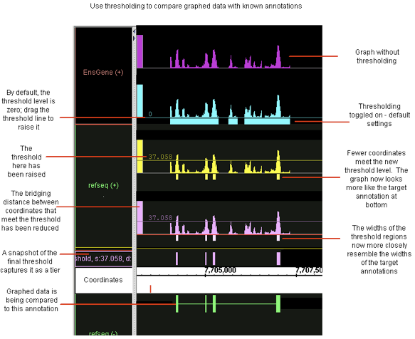
Thresholding displays graph features as annotation-like bars in locations where the graph value at the coordinate meets your defined threshold. You can convert this data into a standard annotation track in order to analyze your graph data using all of the features in IGB for working with and comparing annotations.
In some cases, you may want to adjust your graph thresholds so the bars correlate to existing annotations; any threshold bars visible at that point that don't have known annotation counterparts (or vice-versa) may indicate areas for further investigation.
Using thresholding
To use thresholding:
- Select one or more graphs.
- Click the Thresholding button in the Graph Adjuster tab panel. This will open the Graph Thresholds window.

- Set Visibility to On.
- Modify the thresholding parameters. By default, the threshold is set midway between the graph minimum and maximum values. To obtain more meaningful thresholds, adjust the threshold settings using the methods described in the following sections.
- (Optional) Save the resulting threshold regions to an annotation track by clicking Make Track.
-
- After an annotation track has been created with Make Track, it is frozen and is no longer linked to changes in the Graph Thresholds window. But you are free to modify the criteria in the Graph Thresholds window and create another annotation track.
- Settings in the Graph Thresholds window will apply to all currently-selected graphs.
Specify the threshold level
To change the thresholds of selected graphs so that more or fewer points meet the threshold limit, modify these settings in the Graph Thresholds window:
- By Value – specify the exact threshold value.
- By Percentile – sets the threshold based on the percentage of graph values greater or less than your threshold.
Specify the threshold direction
Specify whether the threshold bars represent values that are above the threshold you specified or below it.
In the Thresholding section of the Graph Adjuster tab, choose:
- > thresh – finds values greater than the specified threshold
- <= thresh – finds values less than or equal to the specified threshold
For example, for expression results graph score represents the level of hybridization activity. For a hybridization activity level to be considered significant, the score must be above a certain threshold. So you would choose the > thresh option and set your desired threshold value. If you need help to pick a threshold level, toggle the Y-axis on to see the graph's scale on the Y-axis. See Graph labeling on page 57.
Control gaps
Experimental data can be noisy. If you are looking for general trends and want to ignore small local variations, you can use the Max Gap and Min run settings.
Slide the sliders to adjust thresholding, or enter values into the boxes for each parameter:
- Max Gap: Groups of coordinates that meet the threshold may be separated by gaps where the threshold is not met. By default, thresholding bridges such gaps if they are less than 100 bps long. For example, if there are 300 bps that meet the threshold, then 99 bps that don't, followed by 100 that do, the threshold bar would bridge the 99 bps to produce a single threshold annotation 499 bps long. To change the length of this bridge, enter a different value into the Max Gap text-entry field.
- Min run: minimum number of bases in a row that must meet the threshold before an annotation bar will appear. For example, by default the Min run is 30 base pairs, so a sequence of 29 base pairs that meet the threshold will not be marked by an annotation bar.
Specify offsets
The Offsets for Thresholded Regions feature is designed specifically for working with tiling array data.
Captured data from tiling array probes should usually be shifted for display. Since the probes are 25 base pairs long, but the x-coordinates given represent the starting coordinate, you should shift the threshold data so that it starts at 12 base pairs past the given beginning, and ends at 13 base pairs past the beginning. This is the default placement of all graph threshold bars.
If these offsets are not correct for the data you are analyzing, you should change them.
If you are viewing typical tiling array data, modify these settings in the Graph Thresholds window:
- Set the Start value to 12.
- Press the <Enter> key.
- Change the End value to 13, then press <Enter>.
When you view non-tiling array data in IGB, you should adjust the offset to 0 to correctly align the threshold bars with their actual coordinates.
To adjust the offset values for non-tiling array data modify these settings in the Graph Thresholds window:
- Set the Start value to 0.
- Press the <Enter> key.
- Change the End value to 1, then press <Enter>.
Capture the threshold bars
Capture the threshold bars (which look similar to annotations) in their own track to more easily compare different threshold settings for a single graphed region. (See the thresholding illustration, above)
To capture the threshold bars and convert them to annotation tracks:
- Click to select the graph
- Click the Make Track button.
A snapshot of the current thresholded graph will be created as a new annotation track. This track will be given a default label which you can later change if desired.
To permanently capture the threshold snapshot for later use or sharing:
- Right-click the track and choose Save Annotations.
- Choose one of the file formats.
- Name your file. Be sure to include the correct filename extension.
After you have captured threshold "annotations" from a graph or other set of data, you can examine these "annotations" using all of the tools in IGB for working with and comparing annotations.
Getting details about a graph
Textual information about some graphs is available in Selection Info.
Click the colored bar at the left of the graph, then click the Selection Info tab. Resize the columns if needed.
Saving and bookmarking graphs
Most graph properties that you set in IGB can be captured for future use by saving or bookmarking.
Saving graph data as a file
You can save a graph as a separate file for future reference or off line use. Note that this saves only the graph data, without any visualization customizations you may have made to it.
To save graph data to a file:
- Select the graph by clicking the colored bar at the left end of the graph.
- Click the Graph Adjuster tab. Click the Save button.
- Specify location and graph name.
- Pick one of the graph formats offered. Typically choose ".egr" format for interval graphs and ".sgr" format for other graphs.
- You will be prompted to add the proper ".sgr" or ".egr" filename extension depending on the type of graph data.
- Click OK.
Graph properties, such as color, scale, and so forth, may not be saved along with the data. Some graph formats, such as ".bed", ".gff", and ".wig" allow such properties to be specified in "track lines".
Bookmarking graph views
By creating a bookmark, you can save a link to your graph along with the customizations you have made to its appearance. See Bookmarking on page 75.
You can also export your list of bookmarks to share it with other users. If your bookmarks contain links to graph files on your file system, those files may not be available to users on other file systems.
Printing graphs
To print directly to your printer:
- Choose File menu > Print.
You can also print to an EPS format file. Files in the EPS format print in high-resolution and can be imported into many graphics programs. Files printed in EPS format are suitable for use in publications. To print to an EPS [file:]
- Choose File menu > Export.
- Choose to export either the Main View or Main View (With Labels)
- Choose a name for your file, using the extension ".eps" .
Setting graph preferences
To set preferences that apply by default when you load graphs, see Setting graph preferences on page 76.