Introduction
A paper published in 2011 titled Utility of RNA Sequencing for Analysis of Maize Reproductive Transcriptomes describes a study that used RNA-Seq to characterize genes expressed in reproductive structures from maize.
About the data
The study sequenced fourteen libraries prepared from fourteen sample types, including pollen, ovules, tassels, anthers, etc. One replicate per sample type was included.
To find out more about the study,
In this tutorial, you'll learn how to load these data into IGB, view genome coverage graphs for a subset of samples, and identify genes that are expressed primarily in ovules, pollen, or other sample types.
To make these data available for visualization in IGB, we downloaded the sequence data from the Short Read Archive and then aligned the sequences onto a maize reference genome assembly using the spliced alignment tool TopHat. We used a program called wiggles (from the TopHat distribute) to generate coverage graph files for each sample. We then set up the files on IGB's QuickLoad site at http://www.igbquickload.org/quickload.
For a description of how we set up the data in the IGB QuickLoad system, please see this page from the IGB Developer's Guide:
What's a coverage graph?
A coverage graph in an RNA-Seq experiment is a type of genome graph that reports the number of reads overlapping regions in the genome. In a coverage graph, the x-coordinates are the genomic base pairs and the y coordinates represent the number of reads overlapping each genomic base.
In this experiment, graphs represent read counts; no normalization has been done. Thus simply comparing graph heights "by eye" can be misleading; you will need to take into account the fact that different samples produced different numbers of mapped reads. However, the number of mapped reads per sample type was similar across the different samples and so the relative heights of coverage graphs can give a reasonably good approximation of gene expression levels per sample.
Here is an example of the first few lines from a bedgraph file:
1 0 6 1
1 6 9 2
1 9 10 4
1 10 35 5
1 35 41 4
The first column reports the name of the sequence (chromosome 1), the next two columns give the start and end coordinates of the first region, and the third number reports the number of reads that overlap that region. Note that the coordinates are in interbase.
- Information about interbase: Introduction to Chado - Interbase Coordinates.
When we processed these data to make them available via IGB QuickLoad, we also computed read alignment distributions for each library. You can view the read alignment distribution files in the same Web directories where the coverage graphs and read alignment files reside. Click the IGB Quickload Data Source to view the data repository and navigate to this folder:
http://igbquickload.org/quickload/Z_mays_B73_Mar_2010/SRP006463/
Setting up
Follow these instructions to configure IGB to get started looking at gene expression in maize reproductive tissues.
- Start IGB
- Download and launch IGB using Java Web Start from http://www.bioviz.org/igb/download.shtml
- Or download igb.zip from http://sourceforge.net/projects/genoviz/files/.
- To launch IGB from igb.zip, double-click igb.zip to unpack it, open folder igb, and double-click run_igb.bat (Windows) or run_igb.command (Mac)
- Choose species Zea mays B73, Genome Version Z_mays_B73_Mar_2010
Note that the gene models for maize should automatically load.
- Customize gene models appearance
- Right-click (or control-click on Mac) the Zea mays gene models track and choose
- Choose Change > Show track (+/-) to combined plus and minus gene models into the same track
- Note that when you zoom in far enough, you'll see arrows appear that indicate the direction of transcription
- Choose Change > Show track (+/-) to combined plus and minus gene models into the same track
- Change background color to white and foreground color to black to maximize readability for printouts and slides
- Right-click (or control-click on Mac) the Zea mays gene models track and choose
Now start opening coverage graphs from different samples from the RNA-Seq experiment.
- Under the Data Access tabbed panel, open
- Data Source IGB Quickload > RNASeq > SRP006463 Reproductive > Single-map reads
- Click the checkboxes next to data sets or click-drag them over to the Data Management Table.
- coverage SRR189770 Ovule
- coverage SRR189771 Pollen
- coverage SRR189766 Embryo
- coverage SRR189761 Leaves
The four data sets will automatically be added to the Data Management Table. Don't worry if you accidentally add a different data set. You can remove it by unchecking the box or clicking the red x.
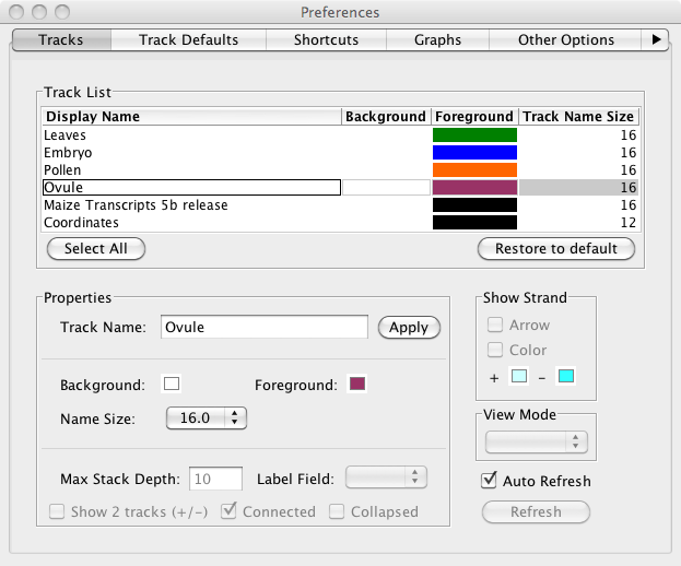
Take a moment to customize the colors. Click the color squares in the Data Management Table (FG is foreground, BG is background) or choose File->Preferences->Tracks to open a new Window that let's you customize different aspects of the display at several at once. Click each row in the table and give each row a white background. Choose colors for individual rows by clicking on them and then selecting options.
Tip: Simplify the track name to make the Track Labels easier to read.
Tip: Color the gene track black (foreground) and white (background) to make attractive images for slides and printing.
Setting IGB Preferences - The preferences window from IGB 6.7.0
Once you've set up the tracks, zoom in on a region.
- Enter 1:51631058-61254530 into the Search/Range Box (upper left corner) and type Return.
IGB should then scroll and zoom to the region you entered. Next, click Load Data and and proceed from the first example below, after adjusting Y-axis scales as described in the next section.
TIP: You can also use IGB links from a Web site to navigate a genome in IGB. An IGB link looks like this: http://localhost:7085/UnibrowControl?seqid=1&end=61254530&start=51631058&version=Z_mays_B73_Mar_2010. When you click the link, IGB should scroll and zoom to the location indicated in the link, provided your computer allows access to non-standard ports. (This may not work on every computer.)
Once the data load, you'll see a view that looks a bit like the image below. To match the image below, you'll need need to rescale the graphs, add a y-axis, and so.
Note to advanced users: If you are running the high-memory version of IGB and have a fast internet connection, you can probably load all the data for chromosome 1 for all four graphs. However, if you try this and out of memory, you can always delete a graph (using the red X) and click the trashcan icon at the bottom right of IGB to force what is called "garbage collection," a programming term that means recovering memory.
Rescale the graphs, add y-axis
Use the Graph Adjuster tab to put all the graphs into the same scale, thus make it possible to compare them. Click the Graph Adjuster tab and then click the Select All button to select all the graphs. While all are selected to the following:
- Click Y Axis to add y axis scale to every graph.
- Unclick Label to hide the label for each graph.
- Under Y-Axis Scale, click By Value and then enter a new maximum. 300 is a good place to start for these data.
- Use the Height slider to increase the height for each graph.
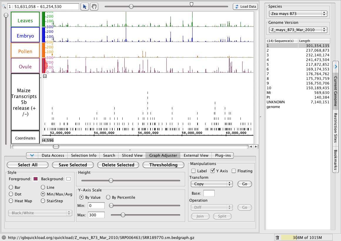
After setting the colors and configuring the Graphs, you should see something like the following image. (The Ovule graph is selected here to show its Graph Adjuster settings.)
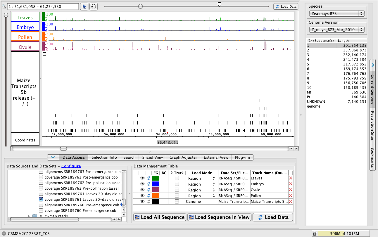
View coverage graphs from four samples
- To jump to this region, enter 1:51631058-61254530 (same as above) into the Search/Range Box (upper left corner) and type Return.
- Click Load Data button (top right) to load the data into IGB.
Explore the data.
Now that the graphs use the same scale, you can zoom and pan around the chromosome and observe how different genes are expressed in different samples.
Use IGB's zoom controls to zoom around in the data
To zoom in, click the place you want to zoom - the vertical stripe (called a zoom stripe) will hop to the location of your most recent click and also will focus zooming so that when you zoom in or out, the zoom stripe will remain stationary while the scene around it expands or contracts. To zoom in, drag the horizontal slider (top right) to the right. To zoom out, drag the horizontal slider to the left.
Stretch the display vertically to show more detail, including gene model labels
To stretch the display in the vertical dimension, drag the the vertical slider (left side of the IGB window) up. To compress the display (and make it fit inside the IGB main data display), drag the vertical slider down.
To zoom in a region, click-drag your mouse along the number line. During the drag, you'll see a blue highlight. When you release the mouse, you'll jump zoom to the region you selected.
Jump-zoom to a gene model by double-clicking on it.
To zoom in on a gene model, just double-click it. This shortcut will help you quickly inspect interesting genes and their structure.
Scroll and zoom around the chromosome, making note of places where one or more samples appear to have more reads covering a particular region and double-click on gene models to zoom in for a closer look.
Also, keep your eyes open for regions with reads but no annotated gene. When you find one, click the corresponding read alignments file for the sample whose graph contained expression data. Load the reads to get an idea of the intron/exon structure for the unannotated gene.
Visit the following regions (see below) to see examples of new genes and differential expression across sample types.
Tip: To navigate quickly to the regions shown below, enter the regions (as shown) in the upper left text box and press the Return key on your keyboard. IGB will then jump to the region you entered. You can also search for gene models by name using the Search tab.
Examples of new genes and/or differential expression across sample types
A multi-kilobase view of chromosome 1
- To jump to this region, paste 1:51,631,058-61,254,530 into the Search/Range box and hit Enter.
Note how different graphs have peaks at different regions, but all graphs use the same scale.
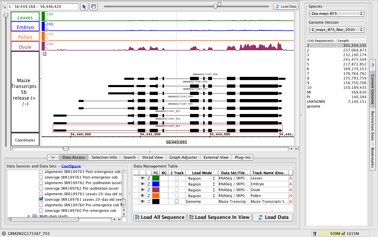
Gene expression high in ovule and lower in leaves and embryo samples.
- To jump to this region, paste 1:56,439,168-56,446,420 into the Search/Range box and hit Enter.
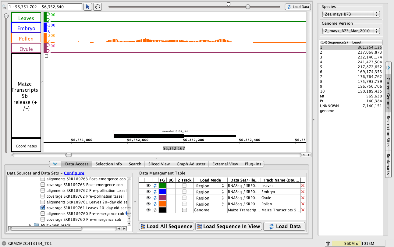
A single-exon gene expressed in pollen but not the other sample types.
- To jump to the region, paste 1:56,351,702-56,352,640 into the Search/Range box and hit Enter.
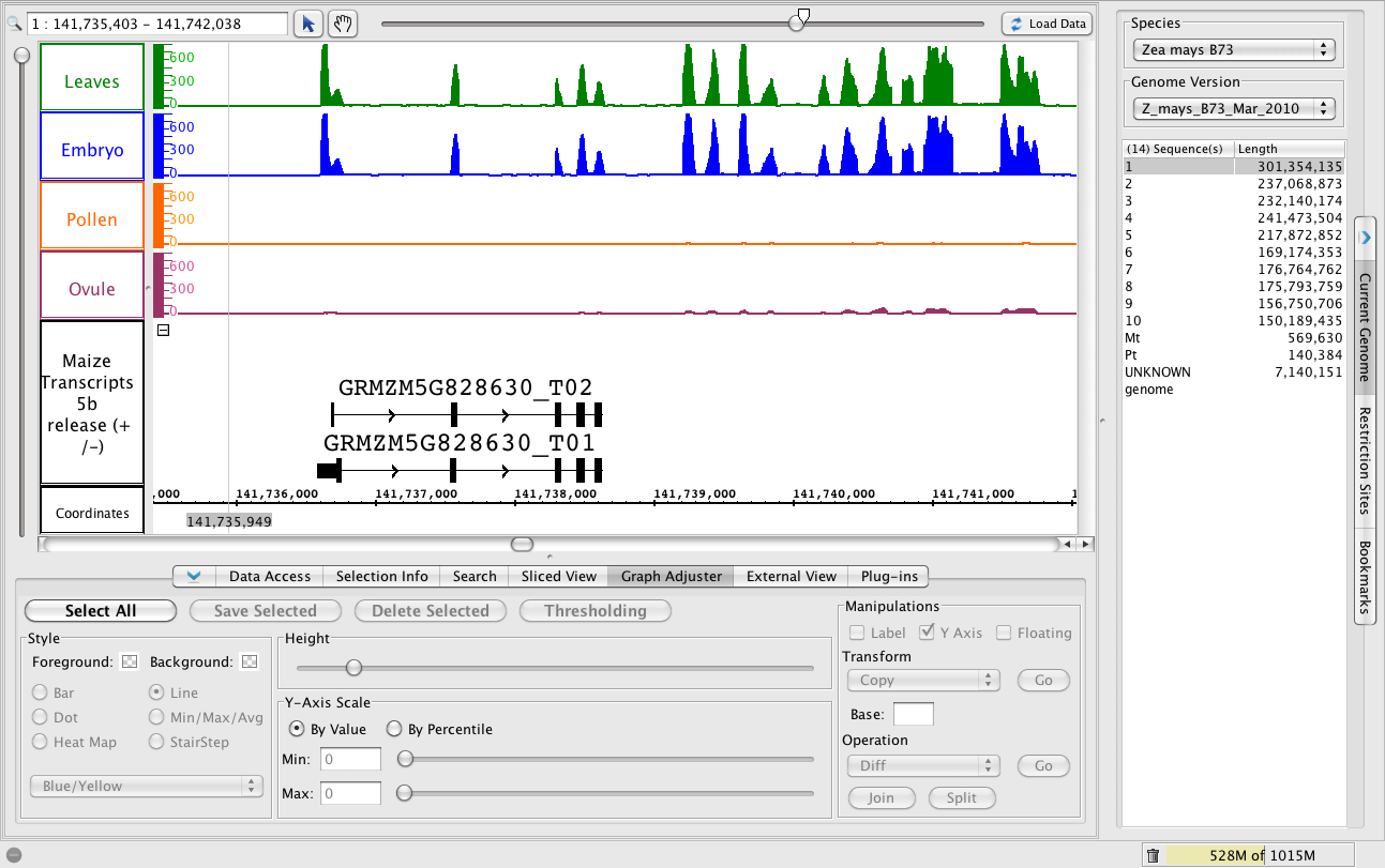
A new gene?
- To jump to the region, paste 1:141,735,403-141,742,038 into the Search/Range box and hit Enter.
- Click Load Data to load the data for this region, which is outside the range of data you loaded earlier in the tutorial.
To replicate this image, modify the Max Stack Depth setting for this track, which controls the amount of vertical space above the two gene models.
- Right-click the Maize Transcripts 5b track label and choose Change > Adjust Max Stack Depth. Enter 2. This will tell IGB to never make a "stack" of individually drawn gene models that is larger than 2. Any other gene models will be drawn on top of each other in the very top row (the "slop" row) at the top of the track.
- When you look at a gene with more than two gene models, use Change > Adjust Max Stack Depth to change this setting to a larger number to see all the gene models individually, or enter 0 to allow unlimited stacking.
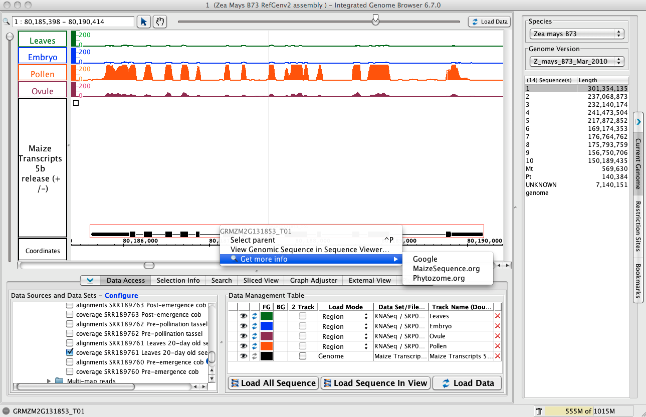
Get more info from Phytozome, maizegenome.org, or google.
- To jump to the region, paste 1:80,185,398-80,190,414 into the Search/Range box and hit Enter.
- Click Load Data to load graphs data for this region, which is outside the first region you loaded.
- Right-click the gene model (as shown below) and choose Get More Info to search Phytozome, MaizeGenome.org, or Google for information about the selected gene.
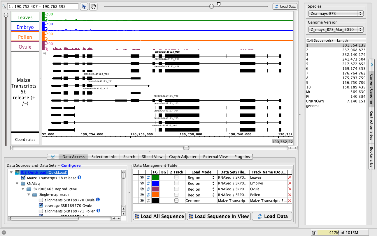
A complex locus with multiple predicted splicing variants.
- To jump to the region, paste 1:190,752,407-190,762,592 into the Search/Range box and hit Enter.
- Click Load Data to load graphs data for the region.
- To view all the variants, change the Max Stack Depth for the track.
- Right-click the Maize transcripts 5b track label and choose Change > Adjust Max Stack Depth. Enter 13 or 0 for unlimited.
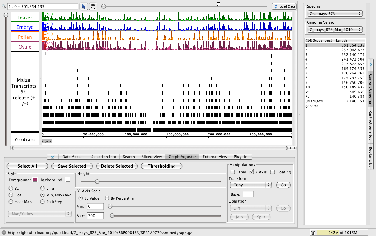
Data loaded for all of chromosome one
- Warning: Loading all of the data from the remote server (igbquickload.org) may take some time! Also, your computer may not have sufficient memory to display all four graphs. But if you would like to try it and view all the data at once, use the horizontal slider (top right) to zoom all the way out. Then, click Load Data. If the loaded data take up too much memory (e.g., close to your maximum memory limit shown on the lower right corner of IGB), then you can delete a data sets by clicking the red X or unchecking it in the Data Sources and Data Sets folder tree.
- To recover memory, click the trash can icon in the bottom right of the display.
- To halt data loading, click the minus symbol that appears in the bottom left whenever data are being accessed from a server or local file.